CNN: Age Estimation and Gender Classification
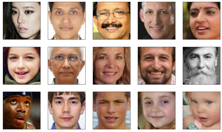
One of the most important applications of Deep Learning is Computer Vision. Today, we will take a deeper dive into this topic and deploy a Convolutional Neural Network (CNN) to predict the age and the gender of faces from the UTKFace dataset.
Dataset
The UTKFace dataset is a large-scale face dataset with an age span from 0 to 116 years old with a resolution of 128x128. However, to avoid long training durations, we will only use a subset of 5,000 images. You can download the dataset by clicking this Link (full dataset can be found on Kaggle).
The project is written in Python and, before starting, make sure to install and import the following libraries.
import numpy as np | |
import os | |
import matplotlib.pyplot as plt | |
from matplotlib.image import imread | |
import glob | |
import random | |
import pandas as pd | |
from sklearn.model_selection import train_test_split | |
from tensorflow.keras.preprocessing.image import ImageDataGenerator | |
from tensorflow.keras.models import Model | |
from tensorflow.keras.layers import Conv2D, MaxPooling2D, Dense, Flatten, Input, Dropout, BatchNormalization | |
from tensorflow.keras.utils import plot_model |
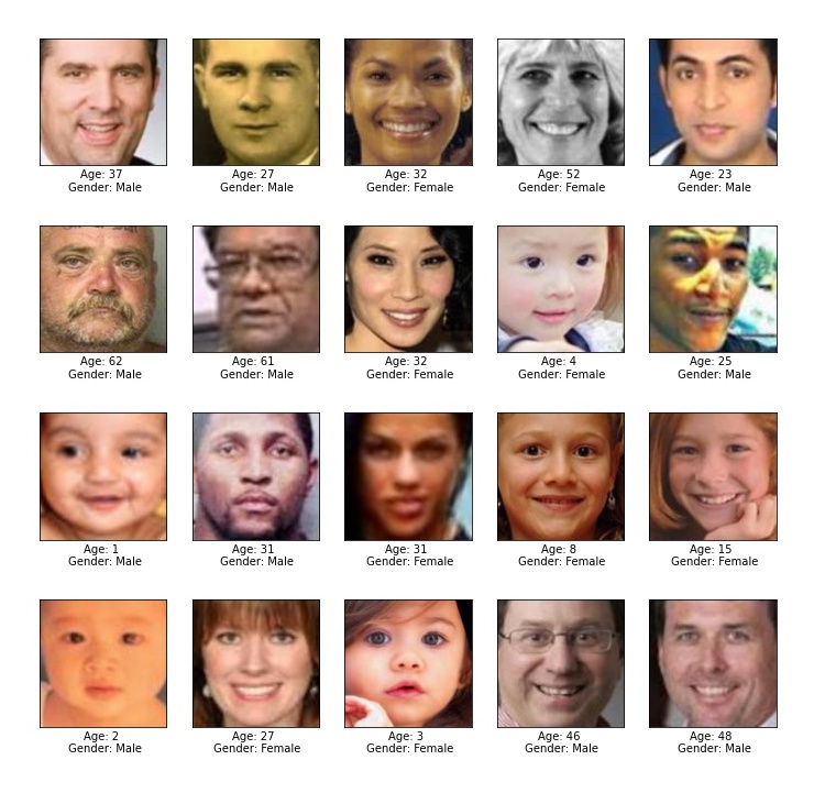
To give you brief idea of how the data looks like, we will first visualise a couple of images. The labels regarding age and gender are hidden in the file name. For instance, the person with the file path train_test/28_1_0_20170117180708809.jpg.chip.jpg
is 28 years old and is female (1 = female, 0 = male).
# get a list of all files in the train_test folder | |
imagepath = (glob.glob('train_test/*')) | |
# plot images | |
plt.figure(figsize=(12,12)) | |
for i in range(20): | |
# add subplots | |
plt.subplot(4,5,i+1) | |
plt.xticks([]) | |
plt.yticks([]) | |
# chose random file | |
filename = random.choice(imagepath) | |
if not os.path.exists(filename): | |
print ('No such file:'+filename) | |
# read image | |
image = imread(filename) | |
plt.imshow(image) | |
# examplary image path: 'train_test/28_1_0_20170117180708809.jpg.chip.jpg' | |
# so we have to split after 11 charcters | |
age = filename[11:].split('_')[0] | |
gender = filename[11:].split('_')[1] | |
# get male and female | |
if gender == '0': | |
gender = 'Male' | |
else: | |
gender = 'Female' | |
plt.xlabel("Age: {} \n Gender: {}".format(age,gender)) | |
plt.show() |
Data Preprocessing
Before we can start with preprocessing, the data needs to be stored in a pandas DataFrame
. Then we can split the data into training and test data, with 20 % being used for testing purposes.
# store important data in a dataframe | |
y_age = [] | |
y_gender = [] | |
for path in imagepath: | |
y_age.append(float(path[11:].split('_')[0])) | |
y_gender.append(int(path[11:].split('_')[1])) | |
df = pd.DataFrame(list(zip(imagepath, y_age, y_gender)), columns=['filename', 'age', 'gender']) | |
df_train, df_val = train_test_split(df, test_size=0.2, random_state=42, stratify=df['gender']) | |
print(df) |
filename age gender
0 train_test/86_1_0_20170120225751953.jpg.chip.jpg 86.0 1
1 train_test/26_1_0_20170116171048641.jpg.chip.jpg 26.0 1
2 train_test/52_0_1_20170117161018159.jpg.chip.jpg 52.0 0
3 train_test/16_0_0_20170104003740977.jpg.chip.jpg 16.0 0
4 train_test/27_0_3_20170119210058457.jpg.chip.jpg 27.0 0
... ... ... ...
4995 train_test/86_1_2_20170105174813405.jpg.chip.jpg 86.0 1
4996 train_test/28_0_2_20170107212142294.jpg.chip.jpg 28.0 0
4997 train_test/1_1_0_20170109194452834.jpg.chip.jpg 1.0 1
4998 train_test/54_0_0_20170109010040814.jpg.chip.jpg 54.0 0
4999 train_test/52_0_3_20170119200211340.jpg.chip.jpg 52.0 0
[5000 rows x 3 columns]
Data Augmentation is an enormously useful tool that is used in most Computer Vision projects. By applying certain variations such as rotation, zoom, or a horizontal flip to the images, it artificially creates new training data from already existing training data
It is so popular mainly due to two big advantages. First, it helps you getting more training data without having to mine new data. Secondly, it is a key tool to prevent overfitting. The model can never fit perfectly on the training data because each epoch you will have slight variations of each image.
The easiest way of implementing Data Augmentation is with the ImageDataGenerator
from tensorflow
. Here, we apply rotation, zoom, and a horizontal flip to our images. Moreover, the rgb value range is scaled to 0 and 1.
# initialise data generator with data augmentation for training data | |
train_datagen = ImageDataGenerator(rescale=1./255, | |
rotation_range = 40, | |
zoom_range = 0.2, | |
horizontal_flip = True) | |
# test data has no augmentation | |
test_datagen = ImageDataGenerator(rescale=1./255) | |
# define batch size | |
batch_size = 20 | |
# generate training batches | |
train_generator = train_datagen.flow_from_dataframe(df_train, | |
y_col=['age', 'gender'], | |
batch_size=batch_size, | |
class_mode='multi_output', | |
target_size=(128, 128)) | |
# generate test batches | |
test_generator = val_datagen.flow_from_dataframe(df_test, y_col=['age', 'gender'], | |
batch_size=batch_size, | |
class_mode='multi_output', | |
target_size=(128, 128)) |
Found 4000 validated image filenames.
Found 1000 validated image filenames.
CNN Model Construction
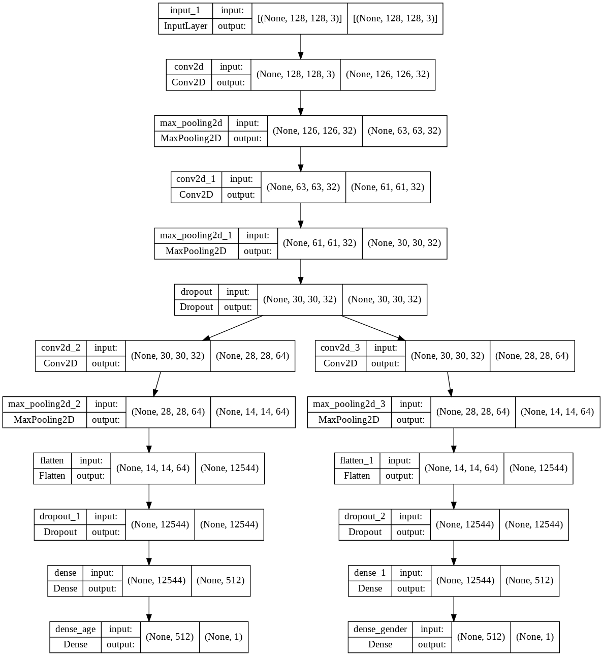
As we are facing a muti-label problem, we need to construct a CNN model that outputs two different values. keras
offers a way to split the model in two at any point of the Neural Network.
Here, two of the three convolutional layers (including padding) are shared between the two branches. After the second convolutional layer, the age and the gender prediction split into two branches. Each of the branches include one more convolutional layer, one dense layer, and one output layer. As you can see below, dropout is also employed in each of the branches and in the shared-learning part.
# input layer | |
input = Input(shape=(128, 128, 3)) | |
# first convolutional layer with padding | |
conv1 = Conv2D(32, (3, 3), activation='relu')(input) | |
maxpool1 = MaxPooling2D((2, 2))(conv1) | |
# second convolutional layer with padding | |
conv2 = Conv2D(32, (3, 3), activation='relu')(maxpool1) | |
maxpool2 = MaxPooling2D((2, 2))(conv2) | |
# add dropout to combat overfitting | |
dropout = Dropout(0.15)(maxpool2) | |
# convolutinoal layer in the age branch | |
conv1_age = Conv2D(64, (3, 3), activation='relu')(dropout) | |
maxpool1_age = MaxPooling2D((2, 2))(conv1_age) | |
# flatten layer | |
flatten_age = Flatten()(maxpool1_age) | |
# dropout | |
dropout_age = Dropout(0.3)(flatten_age) | |
# plot model | |
plot_model(modelA, show_shapes=True) | |
# dense layer | |
dense_age = Dense(512, activation='relu')(dropout_age) | |
# convolutinoal layer in the gender branch | |
conv1_gender = Conv2D(64, (3, 3), activation='relu')(dropout) | |
maxpool1_gender = MaxPooling2D((2, 2))(conv1_gender) | |
# flatten layer | |
flatten_gender = Flatten()(maxpool1_gender) | |
# dropout | |
dropout_gender = Dropout(0.3)(flatten_gender) | |
# dense layer | |
dense_gender = Dense(512, activation='relu')(dropout_gender) | |
# final layer for age estimation | |
out_age = Dense(1, activation='linear', name='dense_age')(dense_age) | |
# final layer for gender classification | |
out_gender = Dense(1, activation='sigmoid', name='dense_gender')(dense_gender) | |
# initialise model | |
modelA = Model(inputs=input, outputs=[out_age, out_gender]) |
Model Training
The following step, obviously, is to train the model. Since the total loss is the sum of the age and the gender loss, we need to make sure that the values of the two loss functions are balanced. Therefore, we weigh the binary_crossentropy
loss of the gender classification 500 times higher than the mse
of the age estimation. The model is trained for 60 epochs.
# compile model | |
modelA.compile(loss={'dense_age':'mse', 'dense_gender':'binary_crossentropy'}, | |
optimizer='adam', | |
loss_weights={'dense_age':1,'dense_gender':500}, # weigh gender more | |
metrics={'dense_age':'mae', 'dense_gender':'accuracy'}) | |
# fit model with 60 epochs | |
history=modelA.fit( | |
train_generator, | |
steps_per_epoch=4000//batch_size, | |
epochs=60, | |
validation_data=val_generator, | |
validation_steps=1000//batch_size) | |
# save model | |
modelA.save("age_gender_A.h5") |
Epoch 1/60
200/200 [==============================] - 15s 73ms/step - loss: 862.1603 - dense_age_loss: 521.0098 - dense_gender_loss: 0.6823 - dense_age_mae: 17.5374 - dense_gender_accuracy: 0.6021 - val_loss: 689.9260 - val_dense_age_loss: 393.1925 - val_dense_gender_loss: 0.5935 - val_dense_age_mae: 14.5779 - val_dense_gender_accuracy: 0.6960
Epoch 2/60
200/200 [==============================] - 14s 72ms/step - loss: 664.3820 - dense_age_loss: 365.3248 - dense_gender_loss: 0.5981 - dense_age_mae: 14.6565 - dense_gender_accuracy: 0.6846 - val_loss: 592.0073 - val_dense_age_loss: 328.2217 - val_dense_gender_loss: 0.5276 - val_dense_age_mae: 13.6442 - val_dense_gender_accuracy: 0.7430
...
Epoch 59/60
200/200 [==============================] - 15s 73ms/step - loss: 275.9303 - dense_age_loss: 138.7035 - dense_gender_loss: 0.2745 - dense_age_mae: 8.8752 - dense_gender_accuracy: 0.8787 - val_loss: 294.9626 - val_dense_age_loss: 132.8631 - val_dense_gender_loss: 0.3242 - val_dense_age_mae: 8.2970 - val_dense_gender_accuracy: 0.8750
Epoch 60/60
200/200 [==============================] - 15s 74ms/step - loss: 266.4663 - dense_age_loss: 129.6572 - dense_gender_loss: 0.2736 - dense_age_mae: 8.6207 - dense_gender_accuracy: 0.8847 - val_loss: 278.6100 - val_dense_age_loss: 122.3719 - val_dense_gender_loss: 0.3125 - val_dense_age_mae: 8.1059 - val_dense_gender_accuracy: 0.8770
Results
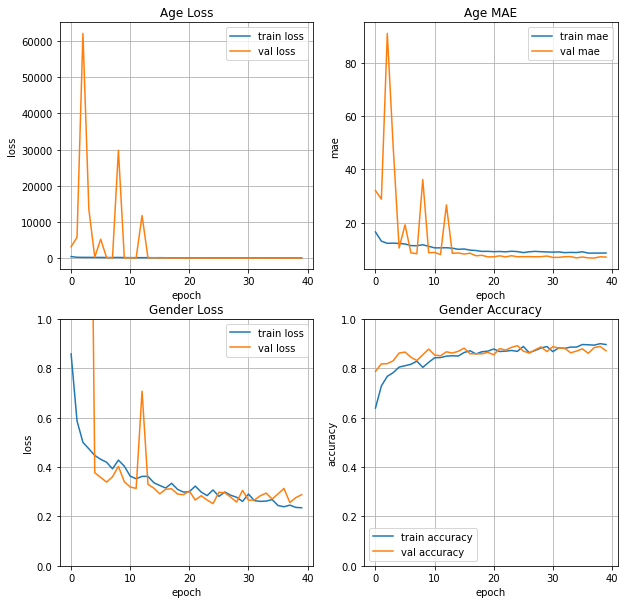
On the test data, the model achieves an 8.11 MAE on age estimation and an 87.70 % accuracy on gender classification. This is a good result, considering the small dataset and the fact that two different variables are predicted in one model.
When we plot the training curves, we can see that due to dropout and data augmentation there is no over- or underfitting present.
# plot training performance | |
# age loss | |
key_list = list(history.history) | |
fig = plt.figure() | |
fig.set_size_inches(12, 12) | |
fig.add_subplot(2,2,1) | |
plt.plot(history.history[key_list[1]], label='train loss') | |
plt.plot(history.history[key_list[6]], label='val loss') | |
plt.legend() | |
plt.grid(True) | |
plt.xlim([0,60]) | |
plt.xlabel('epoch') | |
plt.ylabel('loss') | |
plt.title('Age Loss') | |
# age mae | |
fig.add_subplot(2,2,2) | |
plt.plot(history.history[key_list[3]], label='train mae') | |
plt.plot(history.history[key_list[8]], label='val mae') | |
plt.legend() | |
plt.grid(True) | |
plt.xlim([0,60]) | |
plt.xlabel('epoch') | |
plt.ylabel('mae') | |
plt.title('Age MAE') | |
# gender loss | |
fig.add_subplot(2,2,3) | |
plt.plot(history.history[key_list[2]], label='train loss') | |
plt.plot(history.history[key_list[7]], label='val loss') | |
plt.legend() | |
plt.grid(True) | |
plt.xlim([0,60]) | |
plt.ylim([0,1.0]) | |
plt.xlabel('epoch') | |
plt.ylabel('loss') | |
plt.title('Gender Loss') | |
# gender accuracy | |
fig.add_subplot(2,2,4) | |
plt.plot(history.history[key_list[4]], label='train accuracy') | |
plt.plot(history.history[key_list[9]], label='val accuracy') | |
plt.legend() | |
plt.grid(True) | |
plt.xlim([0,60]) | |
plt.ylim([0.6,1.0]) | |
plt.xlabel('epoch') | |
plt.ylabel('mae') | |
plt.title('Gender accuracy') | |
plt.show() |
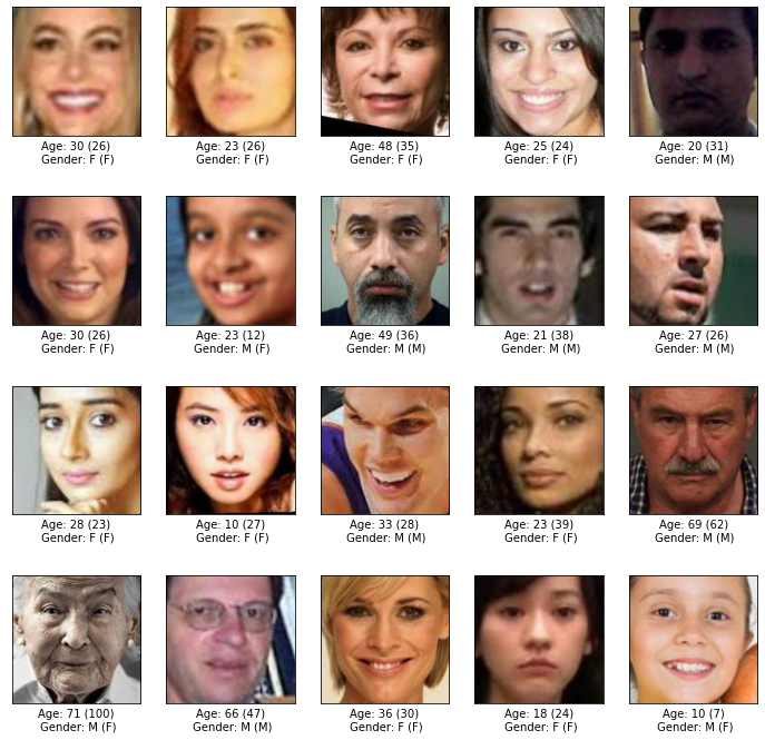
Finally, to give you an idea of how the predictions look like with images present, I sampled 20 images and printed out the prediction with the actual label in brackets. Especially the age estimation would be quite hard even for humans.
# int to string for gender | |
def getGender(gender): | |
if gender == 0: return 'M' | |
else: return'F' | |
# get a sample from test generator and predict | |
i = 0 | |
for batch in test_generator: | |
if i >= 1: | |
break | |
else: | |
X_sample = batch[0] | |
y_sample = batch[1] | |
y_sample_pred = modelA.predict(batch[0]) | |
i = i+1 | |
# plot images | |
random.seed(10) | |
plt.figure(figsize=(12,12)) | |
for i in range(20): | |
# add subplots | |
plt.subplot(4,5,i+1) | |
plt.xticks([]) | |
plt.yticks([]) | |
# plot face | |
plt.imshow(X_sample[i]) | |
# string with prediction and label | |
label = "Age: "+str(round(y_sample_pred[0][i][0]))+" ("+str(round(y_sample[0][i]))+")"+ "\n Gender: "+getGender(round(y_sample_pred[1][i][0]))+" ("+getGender(y_sample[1][i])+")" | |
plt.xlabel(label) | |
plt.show() |